DSB 6200
Term Project Report
XRetailer Supply Chain Network Design Problem Case Study
Contents
DSB 6200 Term Project Report XRetailer Supply Chain
Network Design Problem Case Study
Phase 2: Baseline (As-Is)
Model
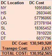
Q1: Total cost of the
network: $130,952,565 (almost $131 million)
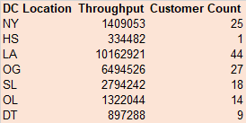
Q2: The below table shows
throughput of each facility:
Q4: Comparison of
throughput levels for each facility compared to baseline:
Q5: Comparison of Scenario
1 Cost to baseline:
Q6: Comparison of
throughput levels for each facility compared to baseline:
Q7: Total Cost of
Scenario 2 and comparison to Total Cost of Scenario 1
Q8: Such a crisis cannot
be perfectly handled within the existing network constraints.
Q9a: If we decide not to
serve some customers:
Q9b: If we decide to
split the quantities as follows:
Q10: What is the best
achievable profit under this scenario?
Files Included
· Final Report (this document)
· PowerPoint Presentation: presented on Friday (submitted previously)
· Excel Model
· GroupBy.html
· Q10-Revenue.html
Phase 1: Preparing Input Data
· Converted all .dat files to .csv using regex via Notepad++
·
GroupBy: HTML file and
Python code (.ipynb) to
combine Customer_Demand and Sku_weight_volume
into one table, drop duplicates, sum at the customer-weight level (to roll up
for use in Excel model), add Kp, and export to new
CSV for use in Excel model
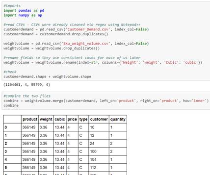
·
Calculated Kp at the
customer-weight level (in Python script) and summed at the customer level for
inclusion in Excel model
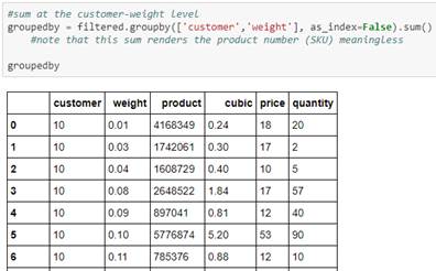
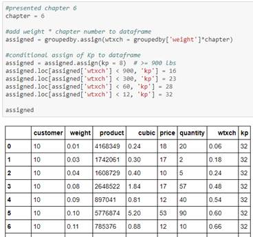
· Quantity summed at the customer level for inclusion in Excel model
· Removed all customers with Quantity of 0 (zero) or 1 – these customers have no demand, so there is no need to ship to them
o 138 customers remained – all are included in Excel model
Phase 2: Baseline (As-Is) Model
Q1: Total cost of the network: $130,952,565 (almost $131 million)
Q2: The below table shows throughput of each
facility:
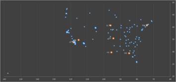
Map of customers (blue) and DCs (orange) weighted by quantity
Q3:
The baseline configuration minimizes Transportation Cost, but may not minimize Total (overall) Cost. DC Cost is much higher than Transportation Cost, so by minimizing Transportation Cost only and treated DC Cost as an afterthought, we are likely not minimizing the Total Cost. There is very likely a lot of missed opportunity to minimize DC Cost.
The major benefit of the baseline configuration is that it is a suboptimal, but still cost-effective, configuration to get the network running and get goods moving while more optimal network designs are calculated and implemented. It also minimizes the travel time from DC to customer, so it’s optimal for getting goods to the customers as quickly as possible from the time they order.
Phase 3: Scenarios
Model Constraints
· Every customer must be served – “satisfy the demand of each customer for each SKU”
o Every customer must be served by at least one DC, but can be served by more than one
· Any DC can serve any customer – except within Phase 2: Baseline (As-Is) Model which is based on minimum distance
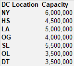
· Max no. of DCs is 6 – “XRetailer can use up to six DCs located in different parts of the network.”
Linearization of Excel Model
·
Properly
speaking, DC Cost should be calculated as:
DC Cost Proper = Fixed Cost + Quantity x Variable Cost
· Total Cost is calculated as: Total Cost = DC Cost Proper + Transportation Cost
· Quantity depends on the Decision Variables in the binary (0/1) to/from matrix
· Variable Cost portion of the calculation depends on Quantity
· However, the Fixed Cost also depends on Quantity because if there is 0 (zero) Quantity, then Fixed Cost must also be 0
· Since Variable Cost and Fixed Cost both depend on Quantity, the objective function is not linear
o When we use Solver or OpenSolver to optimize (minimize) DC Cost Proper, we receive a warning that the objective function is not linear.
o Thus, Total Cost (DC Cost Proper + Transportation Cost) is not linear either and cannot be optimized using Solver/OpenSolver either.
· It is necessary to use linear programming over nonlinear methods to make sure we are calculating the most optimal (minimal) solution for the objective cell
·
To
resolve this problem, we decided to linearize the DC Cost as follows:
DC Cost Linearized = Quantity x New Variable Cost
o
where New Variable Cost is calculated as
follows:
New Variable Cost = Fixed Cost / Capacity + Variable Cost
(Essentially distributing the Fixed Cost across the Capacity of each DC)
· DC Cost Linearized is only dependent once on the Decision Variables (via Quantity) so it is now a linear function; it remains linear when added to Transportation Cost, so Total Cost is linear.
· Evaluating what is lost by linearization: Once Total Cost has been optimized (minimized) as above, then DC Cost Proper (non-linearized DC Cost) can be calculated for the optimized model.
o % Difference between DC Cost Proper and DC Cost Linearized is calculated and displayed in the Excel model
Scenario 1
“relax the requirement that each customer is being sourced from its closest DC”
Q4: Comparison of
throughput levels for each facility compared to baseline:
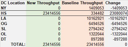
In the baseline configuration, every DC serves at least some customers. In the new configuration, DC_HS serves all customers and it is the only DC in use. HS has a very favorable (low) variable cost, which is why it is preferred. Moreover, the linearization process described earlier further exaggerated the effect of this low variable cost. Nevertheless, as shown below, the Proper cost is even lower than the Linearized cost, so linearization does not change the recommendation to send all material through HS.
Q5: Comparison of Scenario 1 Cost to baseline:
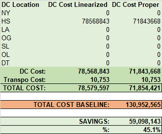
Total Cost in Scenario 1: $71,854,421
Total Cost in Baseline: $130,952,565
Difference: $59,098,143 or 45.1% savings in total network cost
Scenario 2
“limit the maximum quantity that can go out of each DC”
We assumed only one warehouse is allowed at each DC location.
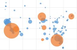
Q6: Comparison of throughput levels for each facility compared to baseline:
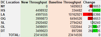
Green bars indicate facilities with more throughput than baseline; red bars
indicate facilities with less throughput than baseline.
NY facility is eliminated due to its higher costs, but all of the others are still in use.
Q7: Total Cost of Scenario 2 and comparison to
Total Cost of Scenario 1
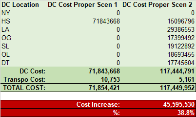
If we limit the maximum quantity that can ship out of each DC as specified in
Scenario 2:
Then costs increase by $45,595,530 or
38.8%. It is still lower-cost than the baseline, but it might be beneficial
for XRetailer to work with the DCs or DC operators to
increase the capacity each DC can handle while maintaining an acceptable level
of product quality. To begin with, XRetailer should
work with the DCs to understand what constraints are currently limiting
capacity, then work on breaking down those constraints.
In fact, the cost difference is so great at almost 40% that it may be prudent for XRetailer to financially assist or loan money to DCs to help with, for example, building additional warehouses or increasing floor space. Such expenses would be one-time costs while DC Costs will continue to add up over every month/year that XRetailer continues to use the DCs.
Scenario 3
“demand would increase by 15%” & “shut down that will make DC_SL, DC_OL, DC_DT unavailable”
Q8: Such a crisis cannot be perfectly handled within the existing network constraints.
We attempted to solve Scenario 3 on top of Scenario 2, but OpenSolver returned “no feasible solution”.
Recommendations and possible solutions:
· Perhaps some customers cannot be served at all and XRetailer will need to weigh the loss of revenues of those contracts and customer retention going forward, versus the cost of continuing to serve those customers – it may be that, on balance, it is financially advised not to serve those customers
· Split quantities per customer: some quantity may go through one DC and the rest through another
· In the real-world, work with DCs to understand constraints limiting capacities and make attempts to increase capacities on remaining DCs while maintaining an acceptable level of product quality
Q9a: If we decide not to serve some customers:
We can solve Scenario 3 on top of Scenario 2, but the following customers can’t be served: 21, 60, 105
Here is the total Quantity, DC Cost, and Total Cost for such a scenario:
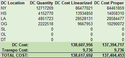
Scenarios 2 and 3 being run simultaneously means maximum DC capacities are limited, SL/OL/DT are unavailable, and demand is increased by 15%. Despite these pressures and constraints being placed on the network, the total network cost is still not much more expensive than the current baseline cost of almost $131 million.
However, again, customers 21, 60, 105 aren’t being served in this case.
Q9b: If we decide to split the quantities as follows:
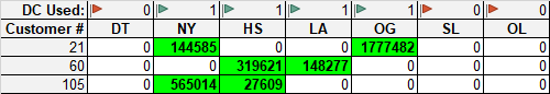
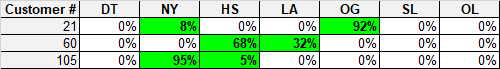
Percentages of quantities, for reference:
This is the closest that OpenSolver can provide to a complete solution without the 0/1 binary constraints on the Decision Variables.
In this case, all customers can be served and all demand can be met, even when maximum DC capacities are limited, SL/OL/DT are unavailable, and demand is increased by 15%.
Here is the total Quantity, DC Cost, and Total Cost for such a scenario:
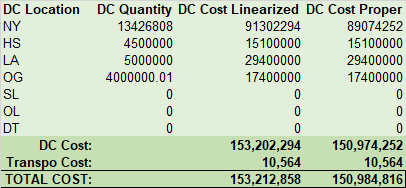
XRetailer would need to decide if serving these three customers is worth an additional $13.5 million in network costs. They may be able to negotiate more revenues from these customers to compensate, in which case they can continue to serve these customers.
Q10: What is the best achievable profit under this scenario?
We do not have revenue information, so we cannot directly calculate profit as revenue minus costs. We attempt to estimate revenue using piece price times quantity. Using the Python script Q10-Revenue, we estimated the total revenue from all SKUs as $118,725,118. Since the above cost of $151 million outweighs the revenue of $119 million, it is not possible to achieve a profit under this scenario.
However, a healthy profit of $46,870,697 is achievable under Scenario 1 and a slight profit of $1,275,166 is achievable under Scenario 2. Thus, again, our primary recommendation to XRetailer is to work with the DCs to understand what constraints are limiting capacities and work to break down those constraints. Without constraints on DC capacity, large profits are possible and XRetailer can be a successful business.